This article needs attention from an expert in statistics. The specific problem is: completion to reasonable standard for probability distributions. (November 2012) |
The Johnson's SU-distribution is a four-parameter family of probability distributions first investigated by N. L. Johnson in 1949.[1][2] Johnson proposed it as a transformation of the normal distribution:[1]
|
Probability density function  | |||
|
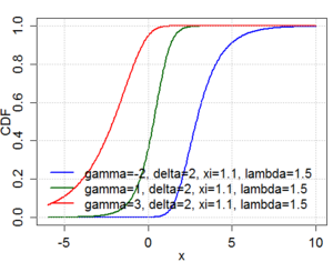
Cumulative distribution function  | |||
| Parameters | (real) | ||
|---|---|---|---|
| Support | |||
| CDF | |||
| Mean | |||
| Median | |||
| Variance | |||
| Skewness | |||
| Excess kurtosis |
| ||
where .
Generation of random variables
editLet U be a random variable that is uniformly distributed on the unit interval [0, 1]. Johnson's SU random variables can be generated from U as follows:
where Φ is the cumulative distribution function of the normal distribution.
Johnson's SB-distribution
editN. L. Johnson[1] firstly proposes the transformation :
where .
Johnson's SB random variables can be generated from U as follows:
The SB-distribution is convenient to Platykurtic distributions (Kurtosis). To simulate SU, sample of code for its density and cumulative distribution function is available here
Applications
editJohnson's -distribution has been used successfully to model asset returns for portfolio management.[3] This comes as a superior alternative to using the Normal distribution to model asset returns. An R package, JSUparameters, was developed in 2021 to aid in the estimation of the parameters of the best-fitting Johnson's -distribution for a given dataset. Johnson distributions are also sometimes used in option pricing, so as to accommodate an observed volatility smile; see Johnson binomial tree.
An alternative to the Johnson system of distributions is the quantile-parameterized distributions (QPDs). QPDs can provide greater shape flexibility than the Johnson system. Instead of fitting moments, QPDs are typically fit to empirical CDF data with linear least squares.
Johnson's -distribution is also used in the modelling of the invariant mass of some heavy mesons in the field of B-physics.[4]
References
edit- ^ a b c Johnson, N. L. (1949). "Systems of Frequency Curves Generated by Methods of Translation". Biometrika. 36 (1/2): 149–176. doi:10.2307/2332539. JSTOR 2332539.
- ^ Johnson, N. L. (1949). "Bivariate Distributions Based on Simple Translation Systems". Biometrika. 36 (3/4): 297–304. doi:10.1093/biomet/36.3-4.297. JSTOR 2332669.
- ^ Tsai, Cindy Sin-Yi (2011). "The Real World is Not Normal" (PDF). Morningstar Alternative Investments Observer.
- ^ As an example, see: LHCb Collaboration (2022). "Precise determination of the – oscillation frequency". Nature Physics. 18: 1–5. arXiv:2104.04421. doi:10.1038/s41567-021-01394-x.
Further reading
edit- Hill, I. D.; Hill, R.; Holder, R. L. (1976). "Algorithm AS 99: Fitting Johnson Curves by Moments". Journal of the Royal Statistical Society. Series C (Applied Statistics). 25 (2).
- Jones, M. C.; Pewsey, A. (2009). "Sinh-arcsinh distributions" (PDF). Biometrika. 96 (4): 761. doi:10.1093/biomet/asp053.( Preprint)
- Tuenter, Hans J. H. (November 2001). "An algorithm to determine the parameters of SU-curves in the Johnson system of probability distributions by moment matching". The Journal of Statistical Computation and Simulation. 70 (4): 325–347. doi:10.1080/00949650108812126. MR 1872992. Zbl 1098.62523.


